catchword
Problem 1
1.1 Problem definition
1.2 Solution of the problem
1.2.1 Linear interpolation
1.2.2 Method of least squares interpolation
1.2.3 Lagrange interpolating polynomial
1.2.4 Cubic spline interpolation
1.3 Results and discussion
1.3.1 Lagrange polynomial
Problem 2
2.1 Problem definition
2.2 Problem solution
2.2.1 Rectangular method
2.2.2 Trapezoidal rule
2.2.3 Simpson's rule
2.2.4 Gauss-Legendre method and Gauss-Chebyshev method
Problem 3
3.1 Problem definition
3.2 Problem solution
Problem 4
4.1 Problem definition
4.2 Problem solution
References
1.1 Problem definition
For the following data set, please discuss the possibility of obtaining a reasonable interpolated value at  , ,  , and , and  via at least 4 different interpolation formulas you are have learned in this semester. via at least 4 different interpolation formulas you are have learned in this semester.


1.2 Solution of the problem
Interpolation is a method of constructing new data points within the range of a discrete set of known data points.
In engineering and science one often has a number of data points, as obtained by sampling or experimentation, and tries to construct a function which closely fits those data points. This is called curve fitting or regression analysis. Interpolation is a specific case of curve fitting, in which the function must go exactly through the data points.
First we have to plot data points, such plot provides better picture for analysis than data arrays
Following four interpolation methods will be discussed in order to solve the problem:
· Linear interpolation
· Method of least squares interpolation
· Lagrange interpolating polynomial

Fig 1. Initial data points
· Cubic spline interpolation
1.2.1 Linear interpolation
One of the simplest methods is linear interpolation (sometimes known as lerp). Generally, linear interpolation tales two data points, say  and and  , and the interpolant is given by: , and the interpolant is given by:
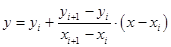 at the point at the point 
Linear interpolation is quick and easy, but it is not very precise/ Another disadvantage is that the interpolant is not differentiable at the point  . .
The method of least squares is an alternative to interpolation for fitting a function to a set of points. Unlike interpolation, it does not require the fitted function to intersect each point. The method of least squares is probably best known for its use in statistical regression, but it is used in many contexts unrelated to statistics.

Fig 2. Plot of the data with linear interpolation superimposed
Generally, if we have  data points, there is exactly one polynomial of degree at most data points, there is exactly one polynomial of degree at most  going through all the data points. The interpolation error is proportional to the distance between the data points to the power n. Furthermore, the interpolant is a polynomial and thus infinitely differentiable. So, we see that polynomial interpolation solves all the problems of linear interpolation. going through all the data points. The interpolation error is proportional to the distance between the data points to the power n. Furthermore, the interpolant is a polynomial and thus infinitely differentiable. So, we see that polynomial interpolation solves all the problems of linear interpolation.
However, polynomial interpolation also has some disadvantages. Calculating the interpolating polynomial is computationaly expensive compared to linear interpolation. Furthermore, polynomial interpolation may not be so exact after all, especially at the end points. These disadvantages can be avoided by using spline interpolation.
Example of construction of polynomial by least square method
Data is given by the table:

Polynomial is given by the model:
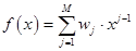
In order to find the optimal parameters 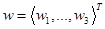 the following substitution is being executed: the following substitution is being executed:
 , ,  , …, , …, 
Then: 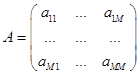
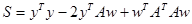
The error function:
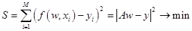
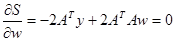
It is necessary to find parameters  , which provide minimums to function , which provide minimums to function  : :

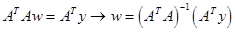
It should be noted that the matrix  must be nonsingular matrix. must be nonsingular matrix.
For the given data points matrix  become singular, and it makes impossible to construct polynomial with become singular, and it makes impossible to construct polynomial with  order, where order, where  - number of data points, so we will use - number of data points, so we will use  polynomial polynomial

Fig 3. Plot of the data with polynomial interpolation superimposed
Because the polynomial is forced to intercept every point, it weaves up and down.
1.2.3 Lagrange interpolating polynomial
The Lagrange interpolating polynomial is the polynomial  of degree of degree  that passes through the points that passes through the points  , ,  , …, , …,  and is given by: and is given by:
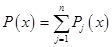 , ,
Where
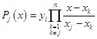
Written explicitly
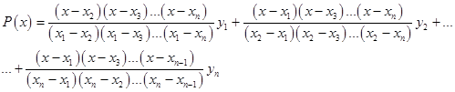
When constructing interpolating polynomials, there is a tradeoff between having a better fit and having a smooth well-behaved fitting function. The more data points that are used in the interpolation, the higher the degree of the resulting polynomial, and therefore the greater oscillation it will exhibit between the data points. Therefore, a high-degree interpolation may be a poor predictor of the function between points, although the accuracy at the data points will be "perfect."

Fig 4. Plot of the data with Lagrange interpolating polynomial interpolation superimposed
One can see, that Lagrange polynomial has a lot of oscillations due to the high order if polynomial.
1.2.4 Cubic spline interpolation
Remember that linear interpolation uses a linear function for each of intervals  . Spline interpolation uses low-degree polynomials in each of the intervals, and chooses the polynomial pieces such that they fit smoothly together. The resulting function is called a spline. For instance, the natural cubic spline is piecewise cubic and twice continuously differentiable. Furthermore, its second derivative is zero at the end points. . Spline interpolation uses low-degree polynomials in each of the intervals, and chooses the polynomial pieces such that they fit smoothly together. The resulting function is called a spline. For instance, the natural cubic spline is piecewise cubic and twice continuously differentiable. Furthermore, its second derivative is zero at the end points.
Like polynomial interpolation, spline interpolation incurs a smaller error than linear interpolation and the interpolant is smoother. However, the interpolant is easier to evaluate than the high-degree polynomials used in polynomial interpolation. It also does not suffer from Runge's phenomenon.

Fig 5. Plot of the data with Lagrange interpolating polynomial interpolation superimposed
It should be noted that cubic spline curve looks like metal ruler fixed in the nodal points, one can see that such interpolation method could not be used for modeling sudden data points jumps.
1.3 Results and discussion
The following results were obtained by employing described interpolation methods for the points  ; ;  ; ;  : :
| Linear interpolation |
Least squares interpolation |
Lagrange polynomial
|
Cubic spline |
Root mean square |
|
0.148 |
0.209 |
0.015 |
0.14 |
0.146 |
|
0.678 |
0.664 |
0.612 |
0.641 |
0.649 |
|
1.569 |
1.649 |
1.479 |
1.562 |
1.566 |
Table 1. Results of interpolation by different methods in the given points.
In order to determine the best interpolation method for the current case should be constructed the table of deviation between interpolation results and root mean square, if number of interpolations methods increases then value of RMS become closer to the true value.
| Linear interpolation |
Least squares interpolation |
Lagrange polynomial |
Cubic spline |
|
 |
 |
 |
 |
|
 |
 |
 |
 |
|
 |
 |
 |
 |
| Average deviation from the RMS |
 |
 |
 |
 |
Table 2. Table of Average deviation between average deviation and interpolation results.
One can see that cubic spline interpolation gives the best results among discussed methods, but it should be noted that sometimes cubic spline gives wrong interpolation, especially near the sudden function change. Also good interpolation results are provided by Linear interpolation method, but actually this method gives average values on each segment between values on it boundaries.
2.1 Problem definition
For the above mentioned data set, if you are asked to give the integration of  between two ends between two ends  and and  ? Please discuss the possibility accuracies of all the numerical integration formulas you have learned in this semester. ? Please discuss the possibility accuracies of all the numerical integration formulas you have learned in this semester.
2.2 Problem solution
In numerical analysis, numerical integration constitutes a broad family of algorithms for calculating the numerical value of a definite integral.
There are several reasons for carrying out numerical integration. The integrand  may be known only at certain points, such as obtained by sampling. Some embedded systems and other computer applications may need numerical integration for this reason. may be known only at certain points, such as obtained by sampling. Some embedded systems and other computer applications may need numerical integration for this reason.
A formula for the integrand may be known, but it may be difficult or impossible to find an antiderivative which is an elementary function. An example of such an integrand is 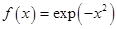 , the antiderivative of which cannot be written in elementary form. , the antiderivative of which cannot be written in elementary form.
It may be possible to find an antiderivative symbolically, but it may be easier to compute a numerical approximation than to compute the antiderivative. That may be the case if the antiderivative is given as an infinite series or product, or if its evaluation requires a special function which is not available.
The following methods were described in this semester:
· Rectangular method
· Trapezoidal rule
· Simpson's rule
· Gauss-Legendre method
· Gauss-Chebyshev method
2.2.1 Rectangular method
The most straightforward way to approximate the area under a curve is to divide up the interval along the x-axis between  and and  into a number of smaller intervals, each of the same length. For example, if we divide the interval into subintervals, then the width of each one will be given by: into a number of smaller intervals, each of the same length. For example, if we divide the interval into subintervals, then the width of each one will be given by:

The approximate area under the curve is then simply the sum of the areas of all the rectangles formed by our subintervals:

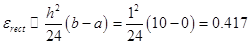
The summary approximation error for intervals with width  is less than or equal to is less than or equal to
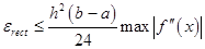
Thus it is impossible to calculate maximum of the derivative function, we can estimate integration error like value:
2.2.2 Trapezoidal rule
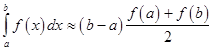
Trapezoidal rule is a way to approximately calculate the definite integral. The trapezium rule works by approximating the region under the graph of the function by a trapezium and calculating its area. It follows that
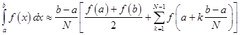
To calculate this integral more accurately, one first splits the interval of integration  into n smaller subintervals, and then applies the trapezium rule on each of them. One obtains the composite trapezium rule: into n smaller subintervals, and then applies the trapezium rule on each of them. One obtains the composite trapezium rule:
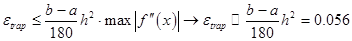
The summary approximation error for intervals with width is less than or equal to:
2.2.3 Simpson's rule
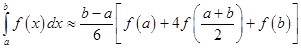
Simpson's rule is a method for numerical integration, the numerical approximation of definite integrals. Specifically, it is the following approximation:
If the interval of integration is in some sense "small", then Simpson's rule will provide an adequate approximation to the exact integral. By small, what we really mean is that the function being integrated is relatively smooth over the interval . For such a function, a smooth quadratic interpolant like the one used in Simpson's rule will give good results.
However, it is often the case that the function we are trying to integrate is not smooth over the interval. Typically, this means that either the function is highly oscillatory, or it lacks derivatives at certain points. In these cases, Simpson's rule may give very poor results. One common way of handling this problem is by breaking up the interval into a number of small subintervals. Simpson's rule is then applied to each subinterval, with the results being summed to produce an approximation for the integral over the entire interval. This sort of approach is termed the composite Simpson's rule.
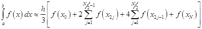
Suppose that the interval is split up in subintervals, with n an even number. Then, the composite Simpson's rule is given by
The error committed by the composite Simpson's rule is bounded (in absolute value) by

2.2.4 Gauss-Legendre method and Gauss-Chebyshev method
Since function values are given in fixed points then just two points Gauss-Legendre method can be applied. If  is continuous on is continuous on  , then , then

The Gauss-Legendre rule  G
2(
f
)
has degree of precision G
2(
f
)
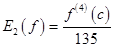
has degree of precision  . If . If  , then , then
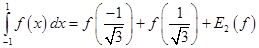 , ,
where
It should be noted that even in case of two points method we have to calculate values of the function in related to  , ,  , this values could be evaluated by linear interpolation (because it is necessary to avoid oscillations), so estimation of integration error become very complicated process, but this error will be less or equal to trapezoidal rule. , this values could be evaluated by linear interpolation (because it is necessary to avoid oscillations), so estimation of integration error become very complicated process, but this error will be less or equal to trapezoidal rule.
Mechanism of Gauss-Chebyshev method is almost the same like described above, and integration error will be almost the same, so there is no reason to use such methods for the current problem.
3.1 Problem definition
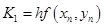
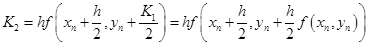
It is well known that the third order Runge-Kutta method is of the following form
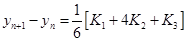 , , 

Suppose that you are asked to derived a new third order Runge-Kutta method in the following from
,
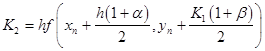

Find determine the unknowns  , ,  , ,  and and  so that your scheme is a third order Runge-Kutta method. so that your scheme is a third order Runge-Kutta method.
3.2 Problem solution
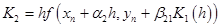
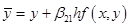
Generally Runge-Kutta method looks like:
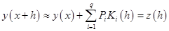 , ,
where coefficients  could be calculated by the scheme: could be calculated by the scheme:

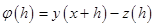
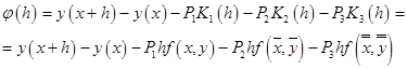
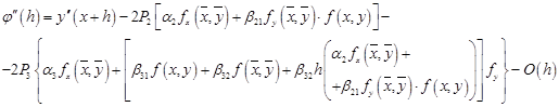
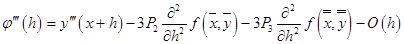
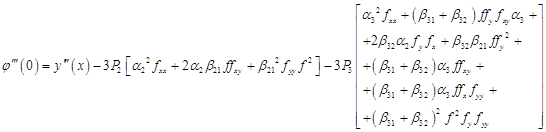
The error function:
Coefficients  , ,  , ,  must be found to satisfy conditions must be found to satisfy conditions 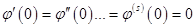 , consequently we can suppose that for each order of Runge-Kutta scheme those coefficients are determined uniquely, it means that there are no two different third order schemes with different coefficients. Now it is necessary to prove statement. , consequently we can suppose that for each order of Runge-Kutta scheme those coefficients are determined uniquely, it means that there are no two different third order schemes with different coefficients. Now it is necessary to prove statement.
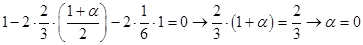
For  , ,  : :
 ; ; 
 ; ; 
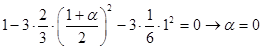
 ; ; 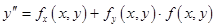 ; ; 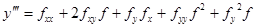


 ; ; 
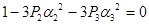 ; ; 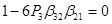 ; ; 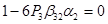
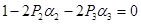
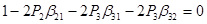
Thus we have system of equations:
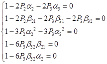
Some of coefficients are already predefined:
 ; ;  ; ;  ; ;  ; ;  ; ;  ; ;  ; ; 
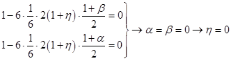
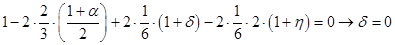
Obtained results show that Runge-Kutta scheme for every order is unique.
Problem 4
4.1 Problem definition
Discuss the stability problem of solving the ordinary equation  , ,  via the Euler explicit scheme via the Euler explicit scheme  , say , say 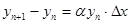 . If . If 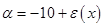 , how to apply your stability restriction? , how to apply your stability restriction?
4.2 Problem solution
The Euler method is 1st order accurate. Given scheme could be rewritten in form of:
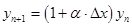
If  has a magnitude greater than one then has a magnitude greater than one then  will tend to grow with increasing and may eventually dominate over the required solution. Hence the Euler method is stable only if will tend to grow with increasing and may eventually dominate over the required solution. Hence the Euler method is stable only if  or: or:
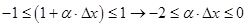
For the case  mentioned above inequality looks like: mentioned above inequality looks like:

Last result shows that integration step mast be less or equal to  . .
For the case 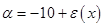 , for the iteration method coefficient looks like , for the iteration method coefficient looks like
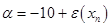
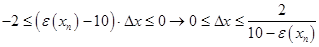
As step  is positive value of the function is positive value of the function  must be less then must be less then  . There are two ways to define the best value of step , the firs one is to define maximum value of function on the integration area, another way is to use different . There are two ways to define the best value of step , the firs one is to define maximum value of function on the integration area, another way is to use different  for each value for each value  , where , where  . So integration step is strongly depends on value of . . So integration step is strongly depends on value of .
1. J. C. Butcher, Numerical methods for ordinary differential equations, ISBN 0471967580
2. George E. Forsythe, Michael A. Malcolm, and Cleve B. Moler. Computer Methods for Mathematical Computations. Englewood Cliffs, NJ: Prentice-Hall, 1977. (See Chapter 6.)
3. Ernst Hairer, Syvert Paul Nørsett, and Gerhard Wanner. Solving ordinary differential equations I: Nonstiff problems, second edition. Berlin: Springer Verlag, 1993. ISBN 3-540-56670-8.
4. William H. Press, Brian P. Flannery, Saul A. Teukolsky, William T. Vetterling. Numerical Recipes in C. Cambridge, UK: Cambridge University Press, 1988. (See Sections 16.1 and 16.2.)
5. Kendall E. Atkinson. An Introduction to Numerical Analysis. John Wiley & Sons - 1989
6. F. Cellier, E. Kofman. Continuous System Simulation. Springer Verlag, 2006. ISBN 0-387-26102-8.
7. Gaussian Quadrature Rule of Integration - Notes, PPT, Matlab, Mathematica, Maple, Mathcad at Holistic Numerical Methods Institute
8. Burden, Richard L.; J. Douglas Faires (2000). Numerical Analysis (7th Ed. ed.). Brooks/Cole. ISBN 0-534-38216-9.
|